Sudoku Solver - Part 3

Hi friends,

Recently I got busy with some other projects, so I couldn't post remaining part.

In the last article, we found the four corners of Sudoku border. In this session, we will be correcting the perspective of Sudoku and making it straight with a uniform size for further works.

So what we have now ? We have four corners of the Sudoku Square. These are the corners, or approx when printed.

[[[491 68]]
[[ 73 84]]
[[ 34 516]]
[[520 522]]]

This is a 4x1x2 array. But check out the values. First row is the TOP-RIGHT corner. Second row is the TOP-LEFT corner. Third row is the BOTTOM-LEFT corner. Finally, fourth one is the BOTTOM-RIGHT corner.

The problem is that, there is no guarantee that for next image, the corners found out will be in this same order. And why should we have the same order?

In the next step, we have to convert these points into another square of size 450x450 such that, the point at [491,68] will be at [449,0] in the new image, similarly for all points. If the order changes, we get some rotated images or even mirrored images.

Therefore , we have to keep them in uniform order. I used this order, [ TOP-LEFT, TOP-RIGHT, BOTTOM-RIGHT, BOTTOM-LEFT ]. You can use whatever you like.

I did it as follows.

First take the sum of x,y coordinates. TOP-LEFT has least sum, and BOTTOM-RIGHT has maximum sum. Now find the difference, ie y-x. TOP-RIGHT has minimum and BOTTOM-LEFT has maximum. It is written as a function. For this, we need to reshape 'approx' to (4,2).

def rectify(h):
        h = h.reshape((4,2))
        hnew = np.zeros((4,2),dtype = np.float32)

        add = h.sum(1)
        hnew[0] = h[np.argmin(add)]
        hnew[2] = h[np.argmax(add)]
        
        diff = np.diff(h,axis = 1)
        hnew[1] = h[np.argmin(diff)]
        hnew[3] = h[np.argmax(diff)]
 
        return hnew

This function should be included at the beginning. Now let's come back to end of code.

approx=rectify(approx)

Now we have the 4 points in order. Now we need corresponding points to where they should be mapped. I took a 450x450 image, and took points as below:

h = np.array([ [0,0],[449,0],[449,449],[0,449] ],np.float32)

Hope it is clear for you. We want the point [ 73 84] to be at [0 0] in new image, point [520 522] should be at [449,449] and so on.

Why image of 450x450 ? Now it has no particular reason, I just took it. 

So earlier ? Yeah, it had some significance back then, when I first trying to develop this. But later I understood it is not needed, and there are more better ways to do it, so gave up the idea,but I retained the size. (Well, that is a little story)

Okay, but why all images should be resized to this ? You will understand it in OCR part. Digits are found using their height and width. So we need all digits to have same size, whatever input image we give.

So now we have the input array (approx) and output array (h). Next we apply the perspective correction.

retval = cv2.getPerspectiveTransform(approx,h)
warp = cv2.warpPerspective(gray,retval,(450,450))

The result is obtained as below :

There is some defects at the top. To correct that also, we need to do some extra efforts, which I will explain in another article.

So we are ready to do OCR work. In next article, I will explain the OCR training.

With Regards,
ARK

Contours - 4 : Ultimate

Hi,

This is the fourth and final article on Contours. This is the continuation of below articles:

1 - Contours - 1 : Getting Started
2 - Contours - 2 : Brotherhood
3 - Contours - 3 : Extraction

In this article we will deal with PointPolygonTest and Convexity Defects.

1 - PointPolygonTest :

This function finds the shortest distance between a point in the image and a contour. It returns the distance which is negative when point is outside the contour, positive when point is inside and zero if point is on the contour.

For example, we can check the point (50,50) as follows:

dist = cv2.pointPolygonTest(cnt,(50,50),True)

In the function, third argument is " measureDist ". If it is True, it finds the signed distance. If False, it finds only if the point is inside or outside or on the contour.

And if you don't want to find the distance, make sure third argument is False, because, it is a time consuming process. So, making it False gives about 2-3X performance boost.

I have written another article on how to speed up programs using Numpy techniques where I have taken PointPolygonTest as the test case.

Visit : Fast Array Manipulation in Numpy

2 - Convexity Defects :

I have already explained convex hull. Any deviation of the object from this hull can be considered as convexity defect. I have explained it with the help of images in second part of this series. ( Please read it ).

OpenCV comes with a ready-made function for this, cv2.convexityDefects(). Let's see how we can use it.

hull = cv2.convexHull(cnt,returnPoints = False)
defects = cv2.convexityDefects(cnt,hull)

Notice that "returnPoints = False" in first line to get indices of the contour points, because input to convexityDefects() should be these indices, not original points.

It returns a defects structure, an array of four values - [ start point, end point, farthest point, approximate distance to farthest point ]

We can visualize it using an image. We draw a line joining start point and end point, then draw a circle at the farthest point.

Now we take each row of the defects, then from that draw, extract four values, draw line using first two values, then draw the point using third value. Remember first three values returned are indices of cnt. So we have to bring those values from cnt.

for i in range(defects.shape[0]):
    s,e,f,d = defects[i,0]
    start = tuple(cnt[s][0])
    end = tuple(cnt[e][0])
    far = tuple(cnt[f][0])
    cv2.line(img,start,end,[0,255,0],2)
    cv2.circle(img,far,5,[0,0,255],-1)

And below are the various results :

So these are two functions I wanted to discuss. With this article, series on Contours is over.

I would like to hear your feedback, comments, suggestions etc.

With Regards,
ARK

Contours - 3 : Extraction

Hi,

This is our third article on contours and direct continuation of Contours 1 : Getting Started and Contours - 2 : Brotherhood. Hope you have read and understood it well before reading this.

In this article, we won't be using any new function from OpenCV, instead we use the methods from previous article to extract useful data of a contour or an object. You will be using some of these routines in your codes often. So we can get into the topic now.

What are these features actually ? Yes, that is a relative question, i think. It can be anything you want to find about an object and it directly depends on your goals. Some times, you may be interested in its size, sometimes its center, or its average color, or minimum and maximum intensity of that object, and even its orientation, ie its slope etc. I would like to list some of the normally used features.

1 - Area and Perimeter :

This, we have already discussed in last articles, which can be found out using cv2.contourArea() and cv2.arcLength() functions, respectively. You can refer that.

2 - Centroid :

Centroids are found using cv2.Moments() function where centroid can be defined as :

centroid_x = M10/M00 and centroid_y = M01/M00

M = cv2.moments(cnt)
centroid_x = int(M['m10']/M['m00'])
centroid_y = int(M['m01']/M['m00'])

Remember, actual result obtained will be 'float', so convert it into 'int'.

If you draw a circle at that point, you can see the centroid.








3 - Aspect Ratio :

Aspect Ratio is the ratio of width to height.

It will be useful in the cases where you want to filter out some shapes. The best example which comes to my mind is ANPR (Automatic Number Plate Recognition). ANPR is used in several traffic surveillance systems to track vehicles going that way. So, in such scenarios, first step is to extract rectangles in the image (since number plate is a rectangle). But there may be false ones also. So use aspect ratio to remove unwanted rectangles (You can google several papers using this method)

x,y,w,h = cv2.boundingRect(cnt)
aspect_ratio = float(w)/h

4 - Extent :

Extent is the ratio of contour area to bounding rectangle area.

area = cv2.contourArea(cnt)
x,y,w,h = cv2.boundingRect(cnt)
rect_area = w*h
extent = float(area)/rect_area

5 - Solidity :

Solidity is the ratio of contour area to its convex hull area.

area = cv2.contourArea(cnt)
hull = cv2.convexHull(cnt)
hull_area = cv2.contourArea(hull)
solidity = float(area)/hull_area

6 - Equivalent Diameter :

Equivalent Diameter is the diameter of the circle whose area is same as the contour area.

It is calculated as, Equivalent Diameter = √ 4 * A / Π 
where A = Area of contour

area = cv2.contourArea(cnt)
equi_diameter = np.sqrt(4*area/np.pi)

7 - Orientation :

Orientation is the angle at which object is directed.

(x,y),(MA,ma),angle = cv2.fitEllipse(cnt)

8 - Pixel Points :

In some cases, we may need all the points which comprises that object. It can be done as follows:

mask = np.zeros(imgray.shape,np.uint8)
cv2.drawContours(mask,[cnt],0,255,-1)
pixelpoints = np.transpose(np.nonzero(mask))

9 - Maximum Value and Minimum Value :

We can find these parameters using a mask image.

min_val, max_val, min_loc,max_loc = cv2.minMaxLoc(imgray,mask = mask)

where mask is same as above. Remember, this is for grayscale images, not for color images.

10 - Mean Color or Mean Intensity :

Here, we can find the average color of an object. Or it can be average intensity of the object in grayscale mode. We again use the same mask to do it.

mean_val = cv2.mean(im,mask = mask)

Remember, if you are trying for color matching or color based object tracking, first convert image to HSV space, because HSV is more better representation of color that RGB space. We will deal it in more detail in another article.

11 - Extreme Points :

Extreme Points means topmost,bottommost,rightmost,leftmost points of the object.

leftmost = tuple(cnt[cnt[:,:,0].argmin()][0])
rightmost = tuple(cnt[cnt[:,:,0].argmax()][0])
topmost = tuple(cnt[cnt[:,:,1].argmin()][0])
bottommost = tuple(cnt[cnt[:,:,1].argmax()][0])

For eg, if I apply it to an Indian map, I get the following result :

Extreme Points

For those who couldn't understand above piece of code, I will explain one for you, ie leftmost.

We have contour points (x,y) stored as a [rows,1,2]. Number of rows equal to number of contour points. So to find the leftmost point, we need to find the point where 'x' is minimum. 'y' doesn't matter. So for that, we extract 'x' coordinates of all the points.

x = cnt[ : , : , 0]

Now we find the location of minimum value in it.( Not minimum value, but position or index of the minimum value)

x_min_loc = x.argmin()

Now we find the point (x,y) in cnt at this location(x_min_loc).

point = cnt[x_min_loc]

Sometimes, there may be more than one leftmost points, like rectangles. So we have to take only one of them. And convert it into tuple.

leftmost = tuple(point[0])

That gives you the answer.

So these are some of the features used frequently.

Now only few more things are there to explain about the contours like convexity defects, point polygon test etc. We will be dealing it in next article.

Send me your feedbacks, comments etc.

Regards,
ARK

Contours - 2 : Brotherhood

Hi,

This article is the direct continuation of this article : Contours - 1: Getting Started

In this article, we will learn usage of several functions closely related to Contours. Once this functions are learnt, we can find almost all features of Contours.

1 - Image Moments

Image moments help you to calculate some features like center of mass of the object, area of the object etc. Check out the wikipedia page : http://en.wikipedia.org/wiki/Image_moment

The function cv2.moments() gives a dictionary of moment values calculated. See below :

moments = cv2.moments(cnt)

If you print moments, you get a dictionary:

{'mu02': 10888082.359906793, 'mu03': 0.005234025965704581, 'm11': 368666693.125,
'nu02': 0.10815497152071127, 'm12': 69763579350.98334, 'mu21': 101313.30416250229, 'mu20': 6674463.831166983,
'nu20': 0.06629968636479547, 'm30': 84692116672.95001, 'nu21': 1.0046975468372928e-05, 'mu11': -1980114.5675549507,
'mu12': -33122544.260385513, 'nu11': -0.019669141689288665, 'nu12': -0.0032846761082870463, 'm02': 352044973.5833333,
'm03': 68983799276.15001, 'm00': 10033.5, 'm01': 1850134.5, 'mu30': 8633090.369003296, 'nu30': 0.0008561209988226333,
'm10': 2010061.8333333333, 'm20': 409360323.5833333, 'm21': 74691021944.88333}

Now you can have calculations using these dictionary keys. For example to find the area of the object:

area = moments['m00']

More we will learn in next article.

2 - Contour Area:

Area of contour is same as number of pixels inside the contour. It can be found out using cv2.contourArea() function.

area = cv2.contourArea(cnt)

3 - Contour Perimeter:

It is also called arc length. It can be found out using cv2.arcLength() function.

perimeter = cv2.arcLength(cnt,True)

4 - Contour Approximation :

Contour Approximation will remove small curves, there by approximating the contour more to straight line. This is done using cv2.approxPolyDP() function.

To understand this, suppose you are trying to find a square in an image, but due to some problems in the image, you got only what is shown at right side.

So when you try to find the contours, you will get all the curves also. But with contour approximation, you can avoid all those problems and approximates it to a perfect square.

Check below image. Red region is the actual contour area. Where green line shows approximated contour. You can see, approximated contour is a perfect rectangle.

approx = cv2.approxPolyDP(cnt,0.1*cv2.arcLength(cnt,True),True)

approximation
epsilon = 10% of arc length

It also reduces number of points to operate. In original contour, there was 210 points, while approximated contour has only four points which corresponds to four corners of rectangle.

In this, second argument is called epsilon, which is maximum distance from contour to approximated contour. It is an accuracy parameter. In above case, i have taken it as 10% of arc length.

approximation
epsilon = 1% of arc length

What will happen if you take it as 1% of arc length? Check out this left image. Approximation detects the defects also. And number of points in approximated contour is now 22.

So a wise selection of epsilon is needed and it all depends on your application.

5 - Convex Hull :

convex hull

Once the approximation is over, Convex Hull is next. This will look similar to contour approximation, but not. Here, cv2.convexHull() function checks a curve for convexity defects and corrects it. Generally speaking, convex curves are the curves which are always bulged out, or at-least flat. And if it is bulged inside, it is called convexity defects. For example, in above case, we can see there are some inside curves for that square. They are the convexity defects. If we find convex hull for this, we get image at right.

(Actually this image is same as above, because both results are same. But it doesn't mean approximation is convex hull, although a contour can be approximated to get a convex hull by selecting suitable epsilon)

Still for those who didn't understand convex hull, OpenCV documentation has a nice picture which demonstrats convex hull and convexity defects. As you can see, the black curve ( hand ) is the original contour. Red curve surrounding it is the convex hull, and convexity defects are marked at gaps between fingers, which are the local maximum deviations of hull from contours.

Syntax :

hull = cv2.convexHull(points[, hull[, clockwise[, returnPoints]]]) 

Points are the contours we pass in to.

Hull is the output, normally we avoid it.

Direction : Orientation flag. If it is true, the output convex hull is oriented clockwise. Otherwise, it is oriented counter-clockwise. (Actually i haven't used this flag anywhere)

So to get a convex hull as in above image, following is sufficient.

hull = cv2.convexHull(cnt)

If we print hull, we get a list: [[[234 202]], [[ 51 202]], [[ 51 79]], [[234 79]]], where each value denotes the corners of rectangle, actually coordinates of corners of rectangle.

To draw a convex hull, you need to do as shown above.

But there is a fourth argument, returnPoints, which is by default True. Then it returns the coordinates. But if it is False, it return the indices of those of convex hull points with respect to contours.

For example, execute the following :

hull = cv2.convexHull(cnt,returnPoints = False)

Now if we print hull, we get : [[129],[ 67],[ 0],[142]]. If you check corresponding values in cnt, it will be same as coordinates we have already found. for example, cnt[129] = [[234, 202]] and so others.

But why would we need such a feature ? It is necessary when we find the convexity defects. We need to pass these indices to cv2.convexityDefects() function to find convexity defects. We will deal with it in another article, but keep this in mind.

6 - Is contour Convex:

There is a function to check if a curve is convex or not, cv2.isContourConvex(). It just return whether True or False. Not a big deal.

k = cv2.isContourConvex(cnt)

7 - Bounding Rectangle :

There are two types of bounding rectangles.

1) Just an upright bounding rectangle which covers the full object. It doesn't consider the rotation of the object.

Let (x,y) be the starting coordinate of rectangle, (w,h) be its width and height.

Then we can find and draw the bounding rect as follows (Green color). See result below:

x,y,w,h = cv2.boundingRect(cnt)
cv2.rectangle(im,(x,y),(x+w,y+h),(0,255,0),2)

2) Rotated rectangle where a bounding rectangle is drawn with minimum area, so it considers the rotation also. The function used is cv2.minAreaRect(). It returns a Box2D structure - (x,y),(w,h),theta.

rect = cv2.minAreaRect(cnt)
box = cv2.cv.BoxPoints(rect)
box = np.int0(box)
cv2.drawContours(im,[box],0,(0,0,255),2)

(x,y) - center point of the box
(w,h) - width and height of the box
theta - angle of rotation

Bounding rectangle

But to draw rectangles, we need coordinate points. For this cv2.cv.BoxPoints() function is used.

Both the rectangles are shown in a single image. Green rectangle shows the normal bounding rect. Red rectangle is the rotated rect.

Area of normal bounding rect = 15972

Area of rotated rect = 8853

CircumCircle

8 - Minimum Enclosing Circle :

Next we find the circumcircle of an object using the function cv2.minEnclosingCircle(). It is a circle which completely covers the object with minimum area.

You can see the result in this image.

(x,y),radius = cv2.minEnclosingCircle(cnt)
center = (int(x),int(y))
radius = int(radius)
cv2.circle(im,center,radius,(0,255,0),2)

9 - Fit Ellipse :

Next one is to fit an ellipse to an object. It returns the rotated rectangle in which the ellipse is inscribed.

ellipse = cv2.fitEllipse(cnt)
cv2.ellipse(im,ellipse,(0,255,0),2)

Fit ellipse

------------------------------------------------------------------------------------------------------------

So, these are some major functions related to Contours.

There are some other functions like, cv2.pointPolygonTest(), cv2.convexityDefects() etc which we will deal in another article.

Hope you like this,

Regards,
ARK

Contours - 1 : Getting Started

Hi, this article is a tutorial which try to cover all relevant functions in OpenCV dealing with Structural Analysis and Shape Descriptors, which are mainly related to contours.

Contours can be explained simply as a curve joining all the continuous points (along the boundary), having same color or intensity. For example, consider image at left.

Assuming it is a binary image,we can say, its contour is the curve joining the all the boundary white points.

So if we find a contour in a binary image, we are finding the boundaries of objects in an image. That is why, OpenCV doc says, "The contours are a useful tool for shape analysis and object detection and recognition".

Finding Contours:

We start with a simple image as above. First we find the contours.

import numpy as np
import cv2

im = cv2.imread('test.jpg')
imgray = cv2.cvtColor(im,cv2.COLOR_BGR2GRAY)
ret,thresh = cv2.threshold(imgray,127,255,0)
contours, hierarchy = cv2.findContours(thresh,cv2.RETR_TREE,cv2.CHAIN_APPROX_SIMPLE)

Points to remember :

1. For better accuracy, use binary images. So before finding contours, apply threshold or canny edge detection.
2. FindContours function modifies the source image, so 'thresh' before and after finding contours are different image. So if you want 'thresh' as such after finding contours, store it to some other variables.
3. In OpenCV, its operation is like finding white object from black background. So remember, object to be found should be white and background in black.

What is structure of resulting contours?

The result "contours" is a Python list, where it contains all objects boundary points as separate lists. So to find number of objects, find length of list "contours", where in this case, it is one. Only one object. So we take it as "cnt".

>>> len(contours)
1
>>> cnt = contours[0]
>>> len(cnt)
244

Here, number of points in cnt is 244. What these points denote? They are the boundary points of the object.

But, does it include all the boundary? Not exactly. The points are selected such that, contours can be drawn as straight line joining these points. So, if object is a horizontal or vertical line, only end points are stored. ie length of cnt = 2. If object is a rectangle, only 4 vertices are stored.

Contour points for a rectangle

Thus in our image, there are no direct horizontal or vertical lines. So most of the points will be stored. To visualise it as above, you can draw circles for each value in cnt.

How to draw the contours?

For this, there is a function, cv2.drawContours(). Let's try it:

cv2.drawContours(im,contours,-1,(0,255,0),3)

This draws a 3-pixel wide green outline of the object. If you want to fill the object with a particular color, pass value of -1 to line thickness.

cv2.drawContours(im,contours,-1,(0,255,0),-1)

Contours drawn filled

Contours drawn 3 px wide

Also, the third argument in cv2.drawContours() is also to be noted. Suppose, you want to draw only fourth contour(not here), third argument should be set to 3. If it is -1, all contours are drawn.

Now you want to draw "cnt" only. It can be done as follows:

cv2.drawContours(im,[cnt],0,(255,0,0),-1)

Note the square bracket around "cnt". Third argument set to 0, means only that particular contour is drawn.

Now we end after one more important concept, called Mask.

Mask : What and Why?

Mask can be considered as a binary image where only our desired area is white and all others are blacked out. They are used to isolate a part of image and do operations on that part only without affecting or operating on other parts of the image. This can also be considered as a ROI (Region of Interest) which can have any shape.

Consider a scenario, where you are asked to find average colors of each shapes in the image at right. So simply threshold the image to binarize it (please don't ask me if white ball can be detected using thresholding, it is just an example). Find contours in the binary image, then for each contour, create a mask image of that shape. ie, if first ball is cosidered, the region of that ball in mask image will be white, while all other shapes and backgrounds are blacked out. Now if you can find the mean color of that shape only. So for every shapes.

(OK, just for this case, I will do it in this image, not on our original image at the beginning)

First we find the contours as we did before. (Adjust the threshold value to detect all). Now we will see how to do it:

First create a mask image where all elements are zero (ie just a black image) with size same as source, but single channel (ie grayscale).

Then for each contour, we draw it on the mask image filled with white color. Then we find mean using mean() function, taking our mask as operating mask.

for h,cnt in enumerate(contours):
    mask = np.zeros(imgray.shape,np.uint8)
    cv2.drawContours(mask,[cnt],0,255,-1)
    mean = cv2.mean(im,mask = mask)

Mask Images

See the result at left side.

(All the resulting images are animated to a single image)

I think it is sufficient for now. Keep these three in mind, ie Find Contours, Draw Contours and Mask Image. Now we can find some contour features in next post.

Regards,
ARK

Fast Array Manipulation in Numpy

Hi,

This post is to explain how fast array manipulation can be done in Numpy. Since we are dealing with images in OpenCV, which are loaded as Numpy arrays, we are dealing with a little big arrays. So we need highly efficient method for fast iteration across this array.

For example, consider an image of size 500x500. If we want to access all the pixels, this itself becomes 250000 calculations. To deal with this, Numpy has got some pretty cool methods. I will explain two of them here, which I know.

For this, I take an example case: You have a 500x500 numpy array of random integers between 0 and 5, ie only 0,1,2,3,4 (just consider you got it as a result of some calculations). These integers actually correspond to different colors like below:

0 ---> Green, [0,255,0]

1 ---> Blue, [255,0,0] // Note that according to OpenCV standards, it is BGR, not RGB

2 ---> Red , [0,0,255]

3 ---> White, [255,255,255]

4 ---> Black, [0,0,0]

So you want to create another 500x500x3 array (or a color image) where integers in x is replaced by corresponding color value.

First of all we deal with our normal method, which is direct indexing method.

What we normally do? Yes, a double loop.

Method 1 : Direct element access

for i in x.rows:
    for j in x.cols:
        check what value at x[i,j]
        put corresponding color in y[i,j]

So that is given below:

First create necessary data, input array 'x', output array 'y', colors etc.

import numpy as np
import time

x = np.random.randint(0,5,(500,500))

green = [0,255,0]
blue = [255,0,0]
red = [0,0,255]
white = [255,255,255]
black = [0,0,0]

rows,cols = x.shape

y = np.zeros((rows,cols,3),np.uint8)  # for output

Now enter the loop:

for i in xrange(rows):
    for j in xrange(cols):
        k = x[i,j]

        if k==0:
            y[i,j] = green

        elif k==1:
            y[i,j] = blue

        elif k==2:
            y[i,j] = red

        elif k==3:
            y[i,j] = white

        else:
            y[i,j] = black

It took about 40-50 seconds to finish the work (I am considering only the loop, and the time depends on the system configuration. So better check at the comparison of results).

Method 2 : Using item() and itemsize()

We normally use k = x[i,j] or x[i,j] = k to read or write an array element. It is very simple, good for large arrays at a single step.

But this style is not at all good for cases like above, where, out of 250000 elements, select each one and modify each one separately. For that, Numpy has got a method to use, ie x.item() to access an element and x.itemset() to write an element. They are much faster than direct accessing. So next we implement our problem using these features ( Only loop portion is given, all others are same):

for i in xrange(rows):
    for j in xrange(cols):
        k = x.item(i,j)

        if k==0:            
            y1.itemset((i,j,0),green[0])
            y1.itemset((i,j,1),green[1])
            y1.itemset((i,j,2),green[2])

 elif k==1:
            y1.itemset((i,j,0),blue[0])
            y1.itemset((i,j,1),blue[1])
            y1.itemset((i,j,2),blue[2])

        elif k==2:
            y1.itemset((i,j,0),red[0])
            y1.itemset((i,j,1),red[1])
            y1.itemset((i,j,2),red[2])

        elif k==3:
            y1.itemset((i,j,0),white[0])
            y1.itemset((i,j,1),white[1])
            y1.itemset((i,j,2),white[2])
            
        else:
            y1.itemset((i,j,0),black[0])
            y1.itemset((i,j,1),black[1])
            y1.itemset((i,j,2),black[2]) 

(Don't be disappointed at the length of code, you will be happy when you see the performance.)

This method took nearly 5 seconds to complete the task. On my calculations, it is around 9-10x faster than the previous method. And that is good result, although length of code is a little problem.

But wait, there is a third method, called palette method.

Method 3 : Palette method

Here, there is no loop. Just three lines of code:

color = [green,blue,red,white,black]
color = np.array(color,np.uint8)
y = color[x]

Finished. See, you can considerably reduce the size of code a lot. And what about performance ? It took less than 0.2 seconds. Just compare the results:

Compared to first method, it is around 350x faster.
Compared to second method, it is around 30-40x faster.

Isn't it good, Reducing the code size to 3 lines, while speeding up the method by more than 300 times? (Truly saying, even I was shocked seeing the performance. I knew it would increase the speed, but never thought this much).

So, to understand what palette methods does and how to utilize it in image processing, we take another experiment with small sample of size 3x3.

Fist take an array of size 3x3 and elements includes only digits (0-9):

>>> a = np.random.randint(0,10,(3,3))
>>> a
array([[9, 8, 4],
       [9, 0, 8],
       [6, 6, 3]])

Next we make another array 'b'. ( You can consider it as the color array).

What should be its rows? It depends on how many color you need. In this example, 'a' has only 9 type of elements (ie digits from 0 to 9) and each corresponds to a color. So we need 9 rows here.

And how many columns ? Are you going for RGB color? Then let there be 3 columns. Or grayscale intensity? Then only one column is sufficient. Here, I take grayscale, so single column,or just an 1-dimensional array.

>>> b = np.random.randint(0,255,10)
>>> b
array([ 97, 177, 237,  29,  51, 230,  92, 198,   6,   7])

See, b[9] = 7. That exactly is happening in palette method. When you type b[a], it actually implies b[i for i in a], ie it takes each element of 'a' and subtitute for 'a' in b[a].

So what ? In our case, when we give c = b[a], it means, c[0,0] = b[ a[0,0] ], ie c[0,0] = b[9] = 7, since a[0,0]=9.

Similarly c[0,1] = b[ a[0,1] ]  ==> c[0,1] = b[8] = 6, and so on. So final result is as follows:

>>> c = b[a]
>>> c
array([[ 7,  6, 51],
       [ 7, 97,  6],
       [92, 92, 29]])

ie, replace every element in 'a' with element in 'b', of which index is decided by the value in 'a'.

Now we need a practical example from image processing. Best example is the PointPolygonTest in OpenCV. First, learn and understand the PointPolygonTest code.

That code, on running, took a minimum of 4.084 seconds (out of 10 runs). Now I removed the part under line 39 in that code and added code as follows, which is a implementation of palette method:

First rounded the values of 'res' to nearest integer.

res = np.int0(np.around(res))

Later, found minimum value in it and multiplied it with 255. Same with maximum also. They are to be used in calculation of color.

mini = res.min()
minie = 255.0/mini

maxi = res.max()
maxie = 255.0/maxi

Now create the image to draw the output. Remember, rows = maximum distance - minimum distance + 1 & columns = 3, for RGB values.

drawing = np.zeros((maxi-mini+1,3),np.uint8)

Now we add minimum distance to the 'res'. It is because, some values in 'res' are negative (distance to point outside contour). So when we apply palette method, negative values will be taken as indices which are not allowed. For that, we add minimum value to all elements in 'res', so that, in new 'res', minimum value is 0.

res = res+abs(mini)

Next part we define the color. For that, we need a single loop, which iterates all the values between res.minimum(mini) and res.maximum(maxi). So, instead of iterating over 160000 values in original method, we just iterate over only less than 300 values (in this case, maxi-mini ≈ ≈ 300). Then coloring scheme is same as in previous method.

for h,i in enumerate(xrange(mini,maxi+1)):
    if i<0:
        drawing.itemset((h,0),255-int(minie*i))
    elif i>0:
        drawing.itemset((h,2),255-int(maxie*i))
    else:
        drawing[h]=[255,255,255]

Now finally apply the palette.

d = drawing[res]

This method took a maximum time of 0.08 seconds (out of 10 runs). That means, it increases the speed by more than 50X. That is a good improvement.

Finally, in this case, although both output look similar, they are not identical. There may be small variations due to rounding off. But it is just a shift of only one pixel and won't be a problem. Look at the results below:

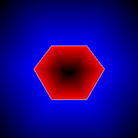
Results in palette method.

Result in normal method

See any difference between both results ? ( If any, it will be negligible compared to performance)

Hope, you enjoyed it. Let me have your feedback.

Regards,
ARK

Image Derivatives and its Applications

Hi,

You can find image derivatives using cv2.Sobel() and cv2.Scharr() functions in OpenCV. There is a nice tutorial and explanation about this in OpenCV site, "Sobel Derivatives". You can find a Python adaptation here:  sobel.py

This post is written to show you some of those functions.





This is the original image →

First I applied Sobel derivatives in vertical and horizontal directions and blended them with equal weights, 0.5. Here is the result →

Next, instead of blending, I directly added them. It gives you a much more bright result, just a fancy development, nothing special →

Next, I applied Scharr instead of Sobel, and again blended them. Here is the result →

Scharr output is considered to be much more accurate.

Next I applied Laplacian operator to the same image. It is sum of second derivatives in both the directions. If you use Sobel to find second derivative and take their sum, you get almost same result. →

You can find tutorial about laplacian operator here: Laplace Operator. You can find corresponding Python implementation here : Python Code

Finally, there is Canny edge detector. Here is the result for canny edge detector for a low threshold value of 74. Original image and edge image is bitwise_and operated to make image a little colorful.

You can find tutorial about canny edge detector here : Canny Edge Detector. Its corresponding Python code is here : Python code

With Regards,
ARK

Sudoku Solver - Part 2

Hi,

This is the continuation of the article : Sudoku Solver - Part 1

So we start implementing here.

Load the image :

Below is the image I used to work with.

Original  Image

So, first we import necessary libraries.

import cv2
import numpy as np

Then we load the image, and convert to grayscale.

img =  cv2.imread('sudoku.jpg')
gray = cv2.cvtColor(img,cv2.COLOR_BGR2GRAY)

Image Pre-processing :

I have done just noise removal and thresholding. And it is working. So I haven't done anything extra.

gray = cv2.GaussianBlur(gray,(5,5),0)
thresh = cv2.adaptiveThreshold(gray,255,1,1,11,2)

Below is the result :

Result of adaptive thresholding

Now two questions may arise :

1) What is the need of smoothing here?
2) Why Adaptive Thresholding ? Why not normal Thresholding using cv2.threshold()  ? 

Find the answers here : Some Common Questions

Find Sudoku Square and Corners :

Now we find the sudoku border. For that, we are taking a practical assumption : The biggest square in the image should be Sudoku Square. In short, image should be taken close to Sudoku, as you can see in the input image of demo.

So a lot of things are clear from this : Image should have only one square, Sudoku Square, or not, Sudoku Square must be the biggest. If this condition is not true, method fails.

It is because, we find the sudoku square by finding the biggest blob ( an independant particle) in the image. So if biggest blob is something other than Sudoku, that blob is processed. So, I think you will keep an eye on it.

We start by finding contours in the thresholded image:

contours, hierarchy = cv2.findContours(thresh, cv2.RETR_TREE, cv2.CHAIN_APPROX_SIMPLE)

Now we find the biggest blob, ie blob with max. area.

For this, first we find area of each blob. Then we filter them by area. We consider a blob for next processing only if its area is greater than a particular value (here, it is 100). If so, we approximate the contours. It removes unwanted coordinate values in the contour and keep only the corners. So if number of corners equal to four, that is a square (actually, a rectangle). If it has the maximum area among all detected squares, it is out Sudoku square.

biggest = None
max_area = 0
for i in contours:
        area = cv2.contourArea(i)
        if area > 100:
                peri = cv2.arcLength(i,True)
                approx = cv2.approxPolyDP(i,0.02*peri,True)
                if area > max_area and len(approx)==4:
                        biggest = approx
                        max_area = area

For you to understand between original contour and approximated contour, I have drawn it on the image (using cv2.drawContours() function). Red line is the original contour, Green line is the approximated contour and corners marked in blue color circles.

Border and corners detected

Look at the top edge of sudoku. Original contour ( Red line) grazes on the edge of square and it is curved. Approximated contour ( Green line) just made it into a straight line.

Now, a simple question may arise. What is the benefit of filtering contours with respect to area? What is the need of removing them ? In simple words, it is done for speed up of the program. Although it may give you a little performance ( in the range of few milliseconds), even that will be good for those who want to implement it in real time. For more explanation, visit : Some Common Questions

Summary :

So, in this section, we have found the boundary of sudoku. Next part is the image transformation. I will explain it in next post.

Until then, I would like to know your feedback, doubts etc.

With Regards
ARK

Sudoku Solver - Some Common Questions

Hi,

This is a post to answer some common questions that can arise while dealing with the Sudoku Solver.

Question 1 : What is the need of Smoothing?

Answer : You will understand its need if you see the result without applying Smoothing. Below is the result of Adaptive Threshold without Smoothing.

Result of adaptive noise without smoothing

You can see the same result after applying a smoothing:

After smoothing

Compare the results. There are lot of noises in the first case. So we have to remove them in the next step which is an extra task.

I just compared number of independent objects found (ie contours ) in both the cases. Below is the result:

First without smoothing:

>>> len(contours)
3109

Next after smoothing:

>>> len(contours)
450

See the difference. Without smoothing, we are dealing with 7 times the number of objects than those found after smoothing. So which one is good?

To know different Smoothing Techniques : Smoothing Techniques in OpenCV

Question 2 : Why adaptive thresholding ? Why not normal thresholding ?

Answer : Reason, You will understand when we compare the results of them. 

Below is the result, I got using Adaptive Threshold :

Result of Adaptive Threshold

Now we apply normal thresholding for a value of 96 ( 96 is the auto threshold value generated by GIMP):

Normal thresholding for value = 96

Now see the difference. It is because normal thresholding thresholds the image taken as a whole, while adaptive threshold thresholds the image taking an optimum value for a local neighbourhood. 

To know more about thresholding techniques :

Question 3 : What is the benefit of filtering contours with respect to area? 

Answer : 1) To avoid small noises which has an area less than prescribed value and we are sure it can't be the square

2) It also improves the speed a little bit.

I will show you some performance comparisons below:

A)  We have already calculated number of objects (contours) found, which is 450. Without having any area filter, it process all the 450 contours. For that, you can just change the code as below:

for i in contours:
    if area > min_size:
        peri = cv2.arcLength(i,True)
        approx = cv2.approxPolyDP(i,0.02*peri,True)
        if area > max_area and len(approx)==4:
            biggest = approx
            max_area = area

It checks all the 450 contours for maximum area and it takes an average of 30 ms.

B)  Now we implement a filter for area of 100, as explained in the original code. Then it takes checks only 100 contours and takes only an average of 15 ms. So we get 2X performance.

C)  Now change the value from 100 to 1/4 of the image size. Check the code below:

min_size = thresh.size/4
for i in contours:
    if area > min_size:
        peri = cv2.arcLength(i,True)
        approx = cv2.approxPolyDP(i,0.02*peri,True)
        if area > max_area and len(approx)==4:
            biggest = approx
            max_area = area

Now it checks only one contour,our square, and takes only an average of 3 ms. ie, 10X performance.

Now, although time difference is only 27 ms, it will be highly useful if we implement it in real time.

So, it all depends on how you use it.

Smoothing Techniques in OpenCV

Hi,

This post is an additional note to official OpenCV tutorial : Smoothing Images

( Its corresponding Python code can be found here : smoothing.py )

Below I would like to show you the results I got when I applied four smoothing techniques in OpenCV, ie cv2.blur, cv2.GaussianBlur, cv2.medianBlur and cv2.bilateralFilter. Kernel size, I used in all cases were 9. See the result below :

Original Image:

Original Image

After Homogeneous Blur, cv2.blur() :

Result of blurring

After Gaussian Blur , cv2.GaussianBlur():

Result of Gaussian Filter

It is much more clear than previous.

After median blur, cv2.medianBlur() :

After median blur

 It has become somewhat like a painting. See eye, it has become completely black.

Finally, after bilateral filter :

This result has high similarity with original image. It is because, it doesn't smooth the edge, instead smooth small noises leaving edges same way. So to see difference, zoom image to left face and check carefully. Then you will understand, face part will have become much more smoother, in short, much more glamorous. There is a nice explanation of bilateral filter at this link : Bilateral Filtering.

But the main problem is that, it takes more time than other filters. 


Regards,
ARK

Difference between Matrix Arithmetic in OpenCV and Numpy

Hi,

This is a small post to show you an important difference in arithmetic operations in OpenCV and Numpy.

As an example,  I take addition as operation.

As you know, images are loaded in OpenCV as "uint8" data. ie 8 bit data. So all the values in the matrix (or image) lie between 0 and 255.

So, even if you add or subtract two numbers, result lies between 0 and 255.

For eg,      255+1 ≠ 256  for 'uint8' data

So what is the answer in above case?

There lies the difference between OpenCV and Numpy. I will demonstrate it using Python terminal.

First create two datas of uint8 type, x = 255, y = 1

>>> x = np.array([255],np.uint8)
>>> y = np.array([1],np.uint8)

OpenCV

Now we add x and y using OpenCV function, cv2.add

>>> cv2.add(x,y)
array([[255]], dtype=uint8)

ie 255+1 = 255 in OpenCV. It is because arithmetic operations in OpenCV are clipped or saturated operations. ie , they clip values wrt data type. If uint8, it clips all values 0 and 255. So if you add two gray pixels, a = 127 and b = 129, you get c = 255, a white pixel, which is OK and necessary in Image Processing

Numpy

Now we add x and y in Numpy.

>>> x+y
array([0], dtype=uint8)

ie 255+1 = 0 in Numpy. It is because Numpy performs a modulo-256 operation. So 256 % 256 = 0.

But what it implies in image processing? If you add a value of  '1' to a white pixel, you get a pure black pixel, which is completely unfavorable in image processing. If you add a = 127 and b = 128, again you get a black pixel.

So better stick to OpenCV functions for image arithmetic operations.

Regards,
ARK

Sudoku Solver - Part 1

Hi,

Now I would like to post a series of tutorials on "Sudoku Solver" .

Actually I started this a few months ago, but got stuck at final part, more specifically, the OCR part. But after a little hacks, I could find a simple method for OCR using kNN. Hope you have read that article  !!!

In this post, I will tell you what exactly I did to develop a "Sudoku Solver".

What exactly it does?

This project on successful completion, accept an image of Sudoku as input, and returns a solved Sudoku back.

See a demonstration below:

Output of sudoku solver

Input Image.

How to accomplish this :

It can be done implementing the methods given in image below :

We will deal with each of one of the steps above:

1. Reading the Image : It is our normal image reading in OpenCV
2. Image Pre-processing : It includes noise removal, brightness/contrast adjustment, thresholding etc. 
3. Find Sudoku Square & Corners : Here we find outer border of Sudoku square and its corners.
4. Image Transformation : Here we reshape irregular Sudoku in input image to a perfect square.
5. Recognize the digit (OCR) : Recognizes the digits in input image and place them in correct position
6. Solve the Sudoku : Here, real solving of Sudoku take place. 
7. Project back the Result : We project the solved Sudoku to image as shown in demo.

In some steps, we take some practical assumptions. One, I would like to tell you now :

The biggest square in the image should be Sudoku Square. In short, image should be taken close to Sudoku, as you can see in the input image of demo. ( Reason, I will tell in upcoming posts).

That is all the theory about this. From next post onwards, we get into practicals on how to implement this.

Waiting for your feedback,

ARK.

Inspired by
1 - Google Goggles Android Application
2 - C++ implementation of Sudoku Solver at Aishack.in
And more...