Saturday, November 30, 2013

Here Comes Official OpenCV-Python Tutorials

Hi,

First of all, our blog visitor count is about to cross 4 lakhs. Thanks to all for your support !!!

So a small gift on this occasion ...

A couple of months ago, I had told you about a new OpenCV-Python tutorial was under development.


So it is the time to unveil it. You can visit the new official tutorial at OpenCV website.

Link : http://docs.opencv.org/trunk/doc/py_tutorials/py_tutorials.html

Remember, it is based on the not-yet-released OpenCV 3.x version. To get it, you have to compile OpenCV from source available in Github. (Because, I always get mail saying some there are some errors in tutorial, it doesn't work. Actually they use OpenCV 2.x version. That is the problem)


It was a great pleasure to work on this project. I thank my mentor, Mr. Alexander Mordvintsev for his help on this project. I also thank many OpenCV developers like Gary Bradsky, Vadim Pisarevsky, Vincent Rabaud etc. for their help.

So friends, please read it, enjoy it, and don't forget to send me your comments, thoughts, feedbacks, bug reports, feature requests etc. I know it is still incomplete. We will together make it complete !!!

Thank you all,

Regards

Abid Rahman K.

Saturday, July 13, 2013

Grabcut Algorithm in OpenCV

Hi friends,

Grabcut algorithm is a nice tool for foreground-background extraction with minimal user interface. It is developed by Microsoft research labs.

See one result below:


You start by drawing a rectangle around the foreground image. Algorithm then segments the image. There can be some misclassifications. There you provide some nice touchups specifying this area is background, this area is foreground etc. Again segment the image to get very nice results.

You can find a python sample at OpenCV source at this link. Watch a video demo of the same code below:


For more details of the algorithm and code, please visit my new tutorial repo: https://github.com/abidrahmank/OpenCV2-Python-Tutorials

Currently, no build is available, so please fork the repo, clone it and build it using sphinx. (Or download zip file if you don't have git account and then build it).

Sphinx installation is just one command with easy_install. Please visit here: http://sphinx-doc.org/

Cheers,
Abid K

Friday, June 7, 2013

" Towards the end of Journey "


Hi friends,

This is a good news or a bad news.

( Bad News ) Most probably, I won't be posting anymore tutorials on this blog.

( Good News ) Within a couple of months, all the tutorials in this blog + a few extra, will be available as online HTML or a PDF document in OpenCV official documentation site (www.docs.opencv.org).

But this time, I am not alone. @Alexander Mordvintsev, a software engineer from Moscow, will be helping me in this journey.


Work is still in its initial stage. Those who want to get a copy of the tutorials, please visit the github repo : https://github.com/abidrahmank/OpenCV2-Python-Tutorials

Fork it, Clone it, Use it.

All details are there in README file. It is created with Sphinx and it looks more better. You will need sphinx to build it.

Since it is in progress, you may find errors and all other unexpected stuffs. Please inform me if you find anyone. You can comment in my blog, you can mail me at abidrahman2@gmail.com, or you can create an issue in git repo.

I will be posting news about development of the work, stay tuned...

Meanwhile, I would like to hear your opinions, comments, feedbacks,... everything :)

Regards

Abid Rahman K.


Sunday, May 19, 2013

Thresholding


Thresholding

Hi friends,

This article is about image thresholding and its different functionalities available in OpenCV. Thresholding converts a grayscale image to a binary image (most of the time). It is highly useful for image segmentation, creating markers, masks etc.

Simple Thresholding


Here, the matter is straight forward. If pixel value is greater than a arbitrary value, it is assigned one value (may be white), else it is assigned another value (may be white).
The function used is threshold(). First param is the source image, which should be a grayscale image. Second param is the threshold value which is used to classify the pixel values. Third param is the maxVal which represents the value to be given if pixel value is more than (sometimes less than) the threshold value. OpenCV provides different styles of thresholding and it decided by the fourth parameter of the function. Different types are:
  1. cv2.THRESH_BINARY
  2. cv2.THRESH_BINARY_INV
  3. cv2.THRESH_TRUNC
  4. cv2.THRESH_TOZERO
  5. cv2.THRESH_TOZERO_INV
Two outputs are obtained. First one is a retval which I will explain later. Second output is our thresholded image.

import cv2
import numpy as np
from matplotlib import pyplot as plt

img = cv2.imread('messi2.jpg',0)
ret,thresh1 = cv2.threshold(img,127,255,cv2.THRESH_BINARY)
ret,thresh2 = cv2.threshold(img,127,255,cv2.THRESH_BINARY_INV)
ret,thresh3 = cv2.threshold(img,127,255,cv2.THRESH_TRUNC)
ret,thresh4 = cv2.threshold(img,127,255,cv2.THRESH_TOZERO)
ret,thresh5 = cv2.threshold(img,127,255,cv2.THRESH_TOZERO_INV)

thresh = ['img','thresh1','thresh2','thresh3','thresh4','thresh5']

for i in xrange(6):
    plt.subplot(2,3,i+1),plt.imshow(eval(thresh[i]),'gray')
    plt.title(thresh[i])

plt.show()

Result :


Adaptive Thresholding


In the previous section, we used a global value as threshold value. But it may not be good in all the conditions where image has different lighting conditions in different areas. In that case, we go for adaptive thresholding. In this, the algorithm calculate the threshold for a small regions of the image. So we get different thresholds for different regions of the same image and it gives us better results for images with varying illumination.
It has three ‘special’ input params and only one output param.
  1. Adaptive Method - It decides how thresholding value is calculated.
    1. cv2.ADAPTIVE_THRESH_MEAN_C : threshold value is the mean of neighbourhood area.
    2. cv2.ADAPTIVE_THRESH_GAUSSIAN_C : threshold value is the weighted sum of neighbourhood values where weights are a gaussian window.
  2. Block Size - It decides the size of neighbourhood area.
  3. C - It is just a constant which is subtracted from the mean or weighted mean calculated.
Below piece of code compares global thresholding and adaptive thresholding for an image with varying illumination.

import cv2
import numpy as np
from matplotlib import pyplot as plt

img = cv2.imread('dave.jpg',0)
img = cv2.medianBlur(img,5)

ret,th1 = cv2.threshold(img,127,255,cv2.THRESH_BINARY)
th2 = cv2.adaptiveThreshold(img,255,cv2.ADAPTIVE_THRESH_MEAN_C,\
            cv2.THRESH_BINARY,11,2)
th3 = cv2.adaptiveThreshold(img,255,cv2.ADAPTIVE_THRESH_GAUSSIAN_C,\
            cv2.THRESH_BINARY,11,2)

plt.subplot(2,2,1),plt.imshow(img,'gray')
plt.title('input image')
plt.subplot(2,2,2),plt.imshow(th1,'gray')
plt.title('Global Thresholding')
plt.subplot(2,2,3),plt.imshow(th2,'gray')
plt.title('Adaptive Mean Thresholding')
plt.subplot(2,2,4),plt.imshow(th3,'gray')
plt.title('Adaptive Gaussian Thresholding')

plt.show()


Otsu’s Binarization


In the first section, I told you there is a second parameter retVal. Its use comes when we go for Otsu’s Binarization. So what is this thing?
In global thresholding, we used an arbitrary value for threshold value, right? So, how can we know a value we selected is good or not? Answer is, trial and error method. But consider a bimodal image. For that image, we can approximately take a value in the middle of those peaks as threshold value, right ? That is what Otsu binarization does.
So in simple words, it automatically calculates a threshold value from image histogram for a bimodal image. (For images which are not bimodal, binarization won’t be accurate.)
For this, our cv2.threshold() function is used, but pass an extra flag, cv2.THRESH_OTSU. For threshold value, simply pass zero. Then the algorithm finds the optimal threshold value and returns you as the second output, retVal. If Otsu thresholding is not used, retVal is same as the threshold value you used.
Check out below example. Input image is a noisy image. First I applied global thresholding for a value of 127. Then I applied Otsu’s thresholding directly. Later I filtered it with a 5x5 gaussian kernel to remove the noise, then applied Otsu thresholding. See how noise filtering improves the result in Figure  [fig:thresh3].

img = cv2.imread('noisy2.png',0)

# global thresholding
ret1,th1 = cv2.threshold(img,127,255,cv2.THRESH_BINARY)

# Otsu's thresholding
ret2,th2 = cv2.threshold(img,0,255,cv2.THRESH_BINARY+cv2.THRESH_OTSU)

# Otsu's thresholding after Gaussian filtering
blur = cv2.GaussianBlur(img,(5,5),0)
ret3,th3 = cv2.threshold(blur,0,255,cv2.THRESH_BINARY+cv2.THRESH_OTSU)

# plot all the images and their histograms
titles = ['img','histogram1','th1',
          'img','histogram2','th2',
          'blur','histogram3','th3']

for i in xrange(3):
    plt.subplot(3,3,i*3+1),plt.imshow(eval(titles[i*3]),'gray')
    plt.title(titles[i*3])
    plt.subplot(3,3,i*3+2),plt.hist(eval(titles[i*3]).ravel(),256)
    plt.title(titles[i*3+1])
    plt.subplot(3,3,i*3+3),plt.imshow(eval(titles[i*3+2]),'gray')
    plt.title(titles[i*3+2])

plt.show()


How Otsu’s Binarization works?


That is very simple. Since we are working with bimodal images, Otsu’s algorithm tries to find a threshold value which minimizes the weighted within-class variance given by the relation :
$$ \sigma_w^2(t) = q_1(t)\sigma_1^2(t)+q_2(t)\sigma_2^2(t) $$
where
$$ q_1(t) = \sum_{i=1}^{t} P(i) \quad \& \quad q_1(t) = \sum_{i=t+1}^{I} P(i) $$
$$ \mu_1(t) = \sum_{i=1}^{t} \frac{iP(i)}{q_1(t)} \quad \& \quad \mu_2(t) = \sum_{i=t+1}^{I} \frac{iP(i)}{q_2(t)} $$
$$ \sigma_1^2(t) = \sum_{i=1}^{t} [i-\mu_1(t)]^2 \frac{P(i)}{q_1(t)} \quad \& \quad \sigma_2^2(t) = \sum_{i=t+1}^{I} [i-\mu_1(t)]^2 \frac{P(i)}{q_2(t)} $$

So our plan is to find the value of $ t $ which minimizes the equation [eq:otsu] and it can be done simply in Numpy as follows :

img = cv2.imread('noisy2.png',0)
blur = cv2.GaussianBlur(img,(5,5),0)

# find normalized_histogram, and its cum_sum
hist = cv2.calcHist([blur],[0],None,[256],[0,256])
hist_norm = hist.ravel()/hist.max()
Q = hist_norm.cumsum()

bins = np.arange(256)

fn_min = np.inf
thresh = -1

for i in xrange(1,256):
    p1,p2 = np.hsplit(hist_norm,[i]) # probabilities
    q1,q2 = Q[i],Q[255]-Q[i] # cum sum of classes
    b1,b2 = np.hsplit(bins,[i]) # weights
    
    # finding means and variances
    m1,m2 = np.sum(p1*b1)/q1, np.sum(p2*b2)/q2 
    v1,v2 = np.sum(((b1-m1)**2)*p1)/q1,np.sum(((b2-m2)**2)*p2)/q2
    
    # calculates the minimization function
    fn = v1*q1 + v2*q2
    if fn < fn_min:
        fn_min = fn
        thresh = i

# find otsu's threshold value with OpenCV function 
ret, otsu = cv2.threshold(blur,0,255,cv2.THRESH_BINARY+cv2.THRESH_OTSU)
print thresh,ret

(There are some optimizations available for this algorithm and that is left for interested people.)

So that's for today. It is a simple and basic tutorial.

Regards,
Abid K.

Thursday, March 14, 2013

Histograms - 4 : Backprojection

Hi friends,

Today, we will look into histogram back-projection. It was proposed by Michael J. Swain , Dana H. Ballard in their paper "Indexing via color histograms".

Well, what is it actually in simple words? It is used for image segmentation or finding objects of interest in an image. In simple words, it creates an image of the same size (but single channel) as that of our input image, where each pixel corresponds to the probability of that pixel belonging to our object. So in short, the output image will have our object of interest in white and remaining part in black. Well, that is an intuitive explanation.

(In this article, I would like to use a beautiful image of a bunch of rose flowers. And the image credit goes to "mi9.com". You can get the image from this link : http://imgs.mi9.com/uploads/flower/4649/rose-flower-wallpaper-free_1920x1080_83181.jpg)

How do we do it ? We create a histogram of an image containing our object of interest (in our case, the rose flower, leaving leaves and background). The object should fill the image as far as possible for better results. And a color histogram is preferred over grayscale histogram, because color of the object is more better way to define the object than its grayscale intensity. ( A red rose flower and its green leaves may have same intensity in grayscale images, but easily distinguishable in color image). We then "back-project" this histogram over our test image where we need to find the object, ie in other words, we calculate the probability of every pixel belonging to rose flower and show it. The resulting output on proper thresholding gives us the rose flower alone.

So let's see how it is done.

Algorithm :

1 - First we need to calculate the color histogram of both the object we need to find (let it be 'M') and the image where we are going to search (let it be 'I').

import cv2
import numpy as np
from matplotlib import pyplot as plt

#roi is the object or region of object we need to find
roi = cv2.imread('rose_red.png')
hsv = cv2.cvtColor(roi,cv2.COLOR_BGR2HSV)

#target is the image we search in
target = cv2.imread('rose.png')
hsvt = cv2.cvtColor(target,cv2.COLOR_BGR2HSV)

# Find the histograms. I used calcHist. It can be done with np.histogram2d also
M = cv2.calcHist([hsv],[0, 1], None, [180, 256], [0, 180, 0, 256] )
I = cv2.calcHist([hsvt],[0, 1], None, [180, 256], [0, 180, 0, 256] )

2 - Find the ratio R = M/I

R = M/(I+1)

3 - Now backproject R, ie use R as palette and create a new image with every pixel as its corresponding probability of being target. ie B(x,y) = R[h(x,y),s(x,y)] where h is hue and s is saturation of the pixel at (x,y). After that apply the condition B(x,y) = min[B(x,y), 1].

h,s,v = cv2.split(hsvt)
B = R[h.ravel(),s.ravel()]
B = np.minimum(B,1)
B = B.reshape(hsvt.shape[:2])

4 - Now apply a convolution with a circular disc, B = D * B, where D is the disc kernel.

disc = cv2.getStructuringElement(cv2.MORPH_ELLIPSE,(5,5))
cv2.filter2D(B,-1,disc,B)
B = np.uint8(B)
cv2.normalize(B,B,0,255,cv2.NORM_MINMAX)

5 - Now the location of maximum intensity gives us the location of object. If we are expecting a region in the image, thresholding for a suitable value gives a nice result.

ret,thresh = cv2.threshold(B,50,255,0)

Below is one example I worked with. I used the region inside blue rectangle as sample object and I wanted to extract all the red roses. See, ROI is filled with red color only :

Histogram Backprojection

Backprojection in OpenCV

OpenCV provides an inbuilt function cv2.calcBackProject(). Its parameters are almost same as the cv2.calcHist() function. One of its parameter is histogram which is histogram of the object and we have to find it. Also, the object histogram should be normalized before passing on to the backproject function. It returns the probability image. Then we convolve the image with a disc kernel and apply threshold. Below is my code and output :

import cv2
import numpy as np

roi = cv2.imread('rose_green.png')
hsv = cv2.cvtColor(img,cv2.COLOR_BGR2HSV)

target = cv2.imread('rose.png')
hsvt = cv2.cvtColor(target,cv2.COLOR_BGR2HSV)

# calculating object histogram
roihist = cv2.calcHist([hsv],[0, 1], None, [180, 256], [0, 180, 0, 256] )

# normalize histogram and apply backprojection
cv2.normalize(roihist,roihist,0,255,cv2.NORM_MINMAX)
dst = cv2.calcBackProject([hsvt],[0,1],roihist,[0,180,0,256],1)

# Now convolute with circular disc
disc = cv2.getStructuringElement(cv2.MORPH_ELLIPSE,(5,5))
cv2.filter2D(dst,-1,disc,dst)

# threshold and binary AND
ret,thresh = cv2.threshold(dst,50,255,0)
thresh = cv2.merge((thresh,thresh,thresh))
res = cv2.bitwise_and(target,thresh)

res = np.vstack((target,thresh,res))
cv2.imwrite('res.jpg',res)

Below is the output. Here ROI is not just flower, but some green part is also included. Still output is good. On close analysis of the center image, you can see the leaf parts slightly which will be removed on threshold :

Histogram Backprojection in OpenCV

Summary

So we have looked on what is Histogram backprojection, how to calculate it, how it is useful in object detection etc. It is also used in more advanced object tracking methods like camshift. We will do that later.

Regards,
Abid Rahman K.

References :

1 - "Indexing via color histograms", Swain, Michael J. , Third international conference on computer vision,1990.
2 - http://www.codeproject.com/Articles/35895/Computer-Vision-Applications-with-C-Part-II
3 - http://theiszm.wordpress.com/tag/backprojection/

Wednesday, March 13, 2013

Histograms - 3 : 2D Histograms

Hi friends,

In the first article, we calculated and plotted one-dimensional histogram. It is called one-dimensional because we are taking only one feature into our consideration, ie grayscale intensity value of the pixel. But in two-dimensional histograms, you consider two features. Normally it is used for finding color histograms where two features are Hue & Saturation values of every pixel.

There is a python sample in the official samples already for finding color histograms. We will try to understand how to create such a color histogram, and it will be useful in understanding further topics like Histogram Back-Projection.

2D Histogram in OpenCV

It is quite simple and calculated using the same function, cv2.calcHist(). For color histogram, we need to convert the image from BGR to HSV. (Remember, for 1D histogram, we converted from BGR to Grayscale). While calling calcHist(), parameters are :

channels = [0,1] # because we need to process both H and S plane.
bins = [180,256] # 180 for H plane and 256 for S plane
range = [0,180,0,256] # Hue value lies between 0 and 180 & Saturation lies between 0 and 256

import cv2
import numpy as np

img = cv2.imread('home.jpg')
hsv = cv2.cvtColor(img,cv2.COLOR_BGR2HSV)

hist = cv2.calcHist( [hsv], [0, 1], None, [180, 256], [0, 180, 0, 256] )

That's it.

2D Histogram in Numpy

Numpy also provides a specific function for this : np.histogram2d(). (Remember, for 1D histogram we used np.histogram() ).

import cv2
import numpy as np
from matplotlib import pyplot as plt

img = cv2.imread('home.jpg')
hsv = cv2.cvtColor(img,cv2.COLOR_BGR2HSV)

hist, xbins, ybins = np.histogram2d(h.ravel(),s.ravel(),[180,256],[[0,180],[0,256]])

First argument is H plane, second one is the S plane, third is number of bins for each and fourth is their range.

Now we can check how to plot this color histogram

Plotting 2D Histogram

Method - 1 : Using cv2.imshow()
The result we get is a two dimensional array of size 180x256. So we can show them as we do normally, using cv2.imshow() function. It will be a grayscale image and it won't give much idea what colors are there, unless you know the Hue values of different colors.

Method - 2 : Using matplotlib
We can use matplotlib.pyplot.imshow() function to plot 2D histogram with different color maps. It gives us much more better idea about the different pixel density. But this also, doesn't gives us idea what color is there on a first look, unless you know the Hue values of different colors. Still I prefer this method. It is simple and better.

NB : While using this function, remember, interpolation flag should be 'nearest' for better results.

import cv2
import numpy as np
from matplotlib import pyplot as plt

img = cv2.imread('home.jpg')
hsv = cv2.cvtColor(img,cv2.COLOR_BGR2HSV)
hist = cv2.calcHist( [hsv], [0, 1], None, [180, 256], [0, 180, 0, 256] )

plt.imshow(hist,interpolation = 'nearest')
plt.show()

Below is the input image and its color histogram plot. X axis shows S values and Y axis shows Hue.

2D Histogram in matplotlib with 'heat' color map


In histogram, you can see some high values near H = 100 and S = 200. It corresponds to blue of sky. Similarly another peak can be seen near H = 25 and S = 100. It corresponds to yellow of the palace. You can verify it with any image editing tools like GIMP.

Method 3 : OpenCV sample style !!
There is a sample code for color_histogram in OpenCV-Python2 samples. If you run the code, you can see the histogram shows even the corresponding color. Or simply it outputs a color coded histogram. Its result is very good (although you need to add extra bunch of lines).

In that code, the author created a color map in HSV. Then converted it into BGR. The resulting histogram image is multiplied with this color map. He also uses some preprocessing steps to remove small isolated pixels, resulting in a good histogram.

I leave it to the readers to run the code, analyze it and have your own hack arounds. Below is the output of that code for the same image as above:

OpenCV-Python sample color_histogram.py output

You can clearly see in the histogram what colors are present, blue is there, yellow is there, and some white due to chessboard(it is part of that sample code) is there. Nice !!!

Summary :

So we have looked into what is 2D histogram, functions available in OpenCV and Numpy, how to plot it etc.

So this is it for today !!!

Regards,
Abid Rahman K.

Tuesday, March 12, 2013

Histograms - 2 : Histogram Equalization


Hi friends,

In last article, we saw what is histogram and how to plot it. This time we can learn a method for image contrast adjustment called "Histogram Equalization".

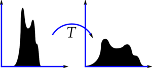
So what is it ? Consider an image whose pixel values are confined to some specific range of values only. For eg, brighter image will have all pixels confined to high values. But a good image will have pixels from all regions of the image. So you need to stretch this histogram to either ends (as given in below image, from wikipedia) and that is what Histogram Equalization does (in simple words). This normally improves the contrast of the image.

Histogram Equalization

Again, I would recommend you to read the wikipedia page on Histogram Equalization for more details about it. It has a very good explanation with worked out examples, so that you would understand almost everything after reading that. And make sure you have checked the small example given in "examples" section before going on to next paragraph.

So, assuming you have checked the wiki page, I will demonstrate a simple implementation of Histogram Equalization with Numpy. After that, I will present you OpenCV function. ( If you are not interested in implementation, you can skip this and go to the end of article)

Numpy Implementation

We start with plotting histogram and its cdf (cumulative distribution function) of the image in Wikipedia page. All the functions are known to us except np.cumsum(). It is used to find the cumulative sum (cdf) of a numpy array.

import cv2
import numpy as np
from matplotlib import pyplot as plt

img = cv2.imread('wiki.jpg',0)

hist,bins = np.histogram(img.flatten(),256,[0,256])

cdf = hist.cumsum()
cdf_normalized = cdf *hist.max()/ cdf.max() # this line not necessary.

plt.plot(cdf_normalized, color = 'b')
plt.hist(img.flatten(),256,[0,256], color = 'r')
plt.xlim([0,256])
plt.legend(('cdf','histogram'), loc = 'upper left')
plt.show()

Input Image and its histogram


You can see histogram lies in brighter region. We need the full spectrum. For that, we need a transformation function which maps the input pixels in brighter region to output pixels in full region. That is what histogram equalization does.

Now we find the minimum histogram value (excluding 0) and apply the histogram equalization equation as given in wiki page. But I have used here, the masked array concept array from Numpy. For masked array, all operations are performed on non-masked elements. You can read more about it from Numpy docs on masked arrays

cdf_m = np.ma.masked_equal(cdf,0)
cdf_m = (cdf_m - cdf_m.min())*255/(cdf_m.max()-cdf_m.min())
cdf = np.ma.filled(cdf_m,0).astype('uint8')

Now we have the look-up table that gives us the information on what is the output pixel value for every input pixel value. So we just apply the transform.

img2 = cdf[img]

Now we calculate its histogram and cdf as before ( you do it) and result looks like below :


Histogram Equalized Image and its histogram


You can see a better contrast in the new image, and it is clear from the histogram also. Also compare the cdfs of two images. First one has a steep slope, while second one is almost a straight line showing all pixels are equi-probable.

Another important feature is that, even if the image was a darker image (instead of a brighter one we used), after equalization we will get almost the same image as we got. As a result, this is used as a "reference tool" (I don't get a more suitable than this) to make all images with same light conditions. This is useful in many cases, for eg, in face recognition, before training the face data, the images of faces are histogram equalized to make them all with same light conditions. It provides better accuracy.

OpenCV Implementation

If you are bored of everything I have written above, just leave them. You need to remember only one function to do this, cv2.calcHist(). Its input is just grayscale image and output is our image.

Below is a simple code snippet showing its usage for same image we used :

img = cv2.imread('wiki.jpg',0)
equ = cv2.equalizeHist(img)
res = np.hstack((img,equ)) #stacking images side-by-side
cv2.imwrite('res.png',res)

See the result :

OpenCV Histogram Equalization


So now you can take different images with different light conditions, equalize it and check the results.

Histogram equalization is good when histogram of the image is confined to a particular region. It won't work good in places where there is large intensity variations where histogram covers a large region, ie both bright and dark pixels are present. I would like to share to SOF questions with you. Please checkout the images in the questions, analyze their histograms, check resulting images after equalization :

How can I adjust contrast in OpenCV in C?
How do I equalize contrast & brightness of images using opencv?

So I would like to wind up this article here. In this article, we learned how to implement Histogram Equalization, how to use OpenCV for that etc. So take images, equalize it and have your own hack arounds.

See you next time !!!
Abid Rahman K.