Histograms - 4 : Backprojection

Hi friends,

Today, we will look into histogram back-projection. It was proposed by Michael J. Swain , Dana H. Ballard in their paper "Indexing via color histograms".

Well, what is it actually in simple words? It is used for image segmentation or finding objects of interest in an image. In simple words, it creates an image of the same size (but single channel) as that of our input image, where each pixel corresponds to the probability of that pixel belonging to our object. So in short, the output image will have our object of interest in white and remaining part in black. Well, that is an intuitive explanation.

(In this article, I would like to use a beautiful image of a bunch of rose flowers. And the image credit goes to "mi9.com". You can get the image from this link : http://imgs.mi9.com/uploads/flower/4649/rose-flower-wallpaper-free_1920x1080_83181.jpg)

How do we do it ? We create a histogram of an image containing our object of interest (in our case, the rose flower, leaving leaves and background). The object should fill the image as far as possible for better results. And a color histogram is preferred over grayscale histogram, because color of the object is more better way to define the object than its grayscale intensity. ( A red rose flower and its green leaves may have same intensity in grayscale images, but easily distinguishable in color image). We then "back-project" this histogram over our test image where we need to find the object, ie in other words, we calculate the probability of every pixel belonging to rose flower and show it. The resulting output on proper thresholding gives us the rose flower alone.

So let's see how it is done.

Algorithm :

1 - First we need to calculate the color histogram of both the object we need to find (let it be 'M') and the image where we are going to search (let it be 'I').

import cv2
import numpy as np
from matplotlib import pyplot as plt

#roi is the object or region of object we need to find
roi = cv2.imread('rose_red.png')
hsv = cv2.cvtColor(roi,cv2.COLOR_BGR2HSV)

#target is the image we search in
target = cv2.imread('rose.png')
hsvt = cv2.cvtColor(target,cv2.COLOR_BGR2HSV)

# Find the histograms. I used calcHist. It can be done with np.histogram2d also
M = cv2.calcHist([hsv],[0, 1], None, [180, 256], [0, 180, 0, 256] )
I = cv2.calcHist([hsvt],[0, 1], None, [180, 256], [0, 180, 0, 256] )

2 - Find the ratio R = M/I

R = M/(I+1)

3 - Now backproject R, ie use R as palette and create a new image with every pixel as its corresponding probability of being target. ie B(x,y) = R[h(x,y),s(x,y)] where h is hue and s is saturation of the pixel at (x,y). After that apply the condition B(x,y) = min[B(x,y), 1].

h,s,v = cv2.split(hsvt)
B = R[h.ravel(),s.ravel()]
B = np.minimum(B,1)
B = B.reshape(hsvt.shape[:2])

4 - Now apply a convolution with a circular disc, B = D * B, where D is the disc kernel.

disc = cv2.getStructuringElement(cv2.MORPH_ELLIPSE,(5,5))
cv2.filter2D(B,-1,disc,B)
B = np.uint8(B)
cv2.normalize(B,B,0,255,cv2.NORM_MINMAX)

5 - Now the location of maximum intensity gives us the location of object. If we are expecting a region in the image, thresholding for a suitable value gives a nice result.

ret,thresh = cv2.threshold(B,50,255,0)

Below is one example I worked with. I used the region inside blue rectangle as sample object and I wanted to extract all the red roses. See, ROI is filled with red color only :

Histogram Backprojection

Backprojection in OpenCV

OpenCV provides an inbuilt function cv2.calcBackProject(). Its parameters are almost same as the cv2.calcHist() function. One of its parameter is histogram which is histogram of the object and we have to find it. Also, the object histogram should be normalized before passing on to the backproject function. It returns the probability image. Then we convolve the image with a disc kernel and apply threshold. Below is my code and output :

import cv2
import numpy as np

roi = cv2.imread('rose_green.png')
hsv = cv2.cvtColor(img,cv2.COLOR_BGR2HSV)

target = cv2.imread('rose.png')
hsvt = cv2.cvtColor(target,cv2.COLOR_BGR2HSV)

# calculating object histogram
roihist = cv2.calcHist([hsv],[0, 1], None, [180, 256], [0, 180, 0, 256] )

# normalize histogram and apply backprojection
cv2.normalize(roihist,roihist,0,255,cv2.NORM_MINMAX)
dst = cv2.calcBackProject([hsvt],[0,1],roihist,[0,180,0,256],1)

# Now convolute with circular disc
disc = cv2.getStructuringElement(cv2.MORPH_ELLIPSE,(5,5))
cv2.filter2D(dst,-1,disc,dst)

# threshold and binary AND
ret,thresh = cv2.threshold(dst,50,255,0)
thresh = cv2.merge((thresh,thresh,thresh))
res = cv2.bitwise_and(target,thresh)

res = np.vstack((target,thresh,res))
cv2.imwrite('res.jpg',res)

Below is the output. Here ROI is not just flower, but some green part is also included. Still output is good. On close analysis of the center image, you can see the leaf parts slightly which will be removed on threshold :

Histogram Backprojection in OpenCV

Summary

So we have looked on what is Histogram backprojection, how to calculate it, how it is useful in object detection etc. It is also used in more advanced object tracking methods like camshift. We will do that later.

Regards,
Abid Rahman K.

References :

1 - "Indexing via color histograms", Swain, Michael J. , Third international conference on computer vision,1990.
2 - http://www.codeproject.com/Articles/35895/Computer-Vision-Applications-with-C-Part-II
3 - http://theiszm.wordpress.com/tag/backprojection/

Histograms - 3 : 2D Histograms

Hi friends,

In the first article, we calculated and plotted one-dimensional histogram. It is called one-dimensional because we are taking only one feature into our consideration, ie grayscale intensity value of the pixel. But in two-dimensional histograms, you consider two features. Normally it is used for finding color histograms where two features are Hue & Saturation values of every pixel.

There is a python sample in the official samples already for finding color histograms. We will try to understand how to create such a color histogram, and it will be useful in understanding further topics like Histogram Back-Projection.

2D Histogram in OpenCV

It is quite simple and calculated using the same function, cv2.calcHist(). For color histogram, we need to convert the image from BGR to HSV. (Remember, for 1D histogram, we converted from BGR to Grayscale). While calling calcHist(), parameters are :

channels = [0,1] # because we need to process both H and S plane.
bins = [180,256] # 180 for H plane and 256 for S plane
range = [0,180,0,256] # Hue value lies between 0 and 180 & Saturation lies between 0 and 256

import cv2
import numpy as np

img = cv2.imread('home.jpg')
hsv = cv2.cvtColor(img,cv2.COLOR_BGR2HSV)

hist = cv2.calcHist( [hsv], [0, 1], None, [180, 256], [0, 180, 0, 256] )

That's it.

2D Histogram in Numpy

Numpy also provides a specific function for this : np.histogram2d(). (Remember, for 1D histogram we used np.histogram() ).

import cv2
import numpy as np
from matplotlib import pyplot as plt

img = cv2.imread('home.jpg')
hsv = cv2.cvtColor(img,cv2.COLOR_BGR2HSV)

hist, xbins, ybins = np.histogram2d(h.ravel(),s.ravel(),[180,256],[[0,180],[0,256]])

First argument is H plane, second one is the S plane, third is number of bins for each and fourth is their range.

Now we can check how to plot this color histogram

Plotting 2D Histogram

Method - 1 : Using cv2.imshow()

The result we get is a two dimensional array of size 180x256. So we can show them as we do normally, using cv2.imshow() function. It will be a grayscale image and it won't give much idea what colors are there, unless you know the Hue values of different colors.

Method - 2 : Using matplotlib

We can use matplotlib.pyplot.imshow() function to plot 2D histogram with different color maps. It gives us much more better idea about the different pixel density. But this also, doesn't gives us idea what color is there on a first look, unless you know the Hue values of different colors. Still I prefer this method. It is simple and better.

NB : While using this function, remember, interpolation flag should be 'nearest' for better results.

import cv2
import numpy as np
from matplotlib import pyplot as plt

img = cv2.imread('home.jpg')
hsv = cv2.cvtColor(img,cv2.COLOR_BGR2HSV)
hist = cv2.calcHist( [hsv], [0, 1], None, [180, 256], [0, 180, 0, 256] )

plt.imshow(hist,interpolation = 'nearest')
plt.show()

Below is the input image and its color histogram plot. X axis shows S values and Y axis shows Hue.

2D Histogram in matplotlib with 'heat' color map

In histogram, you can see some high values near H = 100 and S = 200. It corresponds to blue of sky. Similarly another peak can be seen near H = 25 and S = 100. It corresponds to yellow of the palace. You can verify it with any image editing tools like GIMP.

Method 3 : OpenCV sample style !!

There is a sample code for color_histogram in OpenCV-Python2 samples. If you run the code, you can see the histogram shows even the corresponding color. Or simply it outputs a color coded histogram. Its result is very good (although you need to add extra bunch of lines).

In that code, the author created a color map in HSV. Then converted it into BGR. The resulting histogram image is multiplied with this color map. He also uses some preprocessing steps to remove small isolated pixels, resulting in a good histogram.

I leave it to the readers to run the code, analyze it and have your own hack arounds. Below is the output of that code for the same image as above:

OpenCV-Python sample color_histogram.py output

You can clearly see in the histogram what colors are present, blue is there, yellow is there, and some white due to chessboard(it is part of that sample code) is there. Nice !!!

Summary :

So we have looked into what is 2D histogram, functions available in OpenCV and Numpy, how to plot it etc.

So this is it for today !!!

Regards,
Abid Rahman K.

Histograms - 2 : Histogram Equalization

Hi friends,

In last article, we saw what is histogram and how to plot it. This time we can learn a method for image contrast adjustment called "Histogram Equalization".

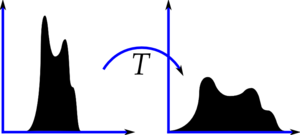
So what is it ? Consider an image whose pixel values are confined to some specific range of values only. For eg, brighter image will have all pixels confined to high values. But a good image will have pixels from all regions of the image. So you need to stretch this histogram to either ends (as given in below image, from wikipedia) and that is what Histogram Equalization does (in simple words). This normally improves the contrast of the image.

Histogram Equalization

Again, I would recommend you to read the wikipedia page on Histogram Equalization for more details about it. It has a very good explanation with worked out examples, so that you would understand almost everything after reading that. And make sure you have checked the small example given in "examples" section before going on to next paragraph.

So, assuming you have checked the wiki page, I will demonstrate a simple implementation of Histogram Equalization with Numpy. After that, I will present you OpenCV function. ( If you are not interested in implementation, you can skip this and go to the end of article)

Numpy Implementation

We start with plotting histogram and its cdf (cumulative distribution function) of the image in Wikipedia page. All the functions are known to us except np.cumsum(). It is used to find the cumulative sum (cdf) of a numpy array.

import cv2
import numpy as np
from matplotlib import pyplot as plt

img = cv2.imread('wiki.jpg',0)

hist,bins = np.histogram(img.flatten(),256,[0,256])

cdf = hist.cumsum()
cdf_normalized = cdf *hist.max()/ cdf.max() # this line not necessary.

plt.plot(cdf_normalized, color = 'b')
plt.hist(img.flatten(),256,[0,256], color = 'r')
plt.xlim([0,256])
plt.legend(('cdf','histogram'), loc = 'upper left')
plt.show()

Input Image and its histogram

You can see histogram lies in brighter region. We need the full spectrum. For that, we need a transformation function which maps the input pixels in brighter region to output pixels in full region. That is what histogram equalization does.

Now we find the minimum histogram value (excluding 0) and apply the histogram equalization equation as given in wiki page. But I have used here, the masked array concept array from Numpy. For masked array, all operations are performed on non-masked elements. You can read more about it from Numpy docs on masked arrays

cdf_m = np.ma.masked_equal(cdf,0)
cdf_m = (cdf_m - cdf_m.min())*255/(cdf_m.max()-cdf_m.min())
cdf = np.ma.filled(cdf_m,0).astype('uint8')

Now we have the look-up table that gives us the information on what is the output pixel value for every input pixel value. So we just apply the transform.

img2 = cdf[img]

Now we calculate its histogram and cdf as before ( you do it) and result looks like below :

Histogram Equalized Image and its histogram

You can see a better contrast in the new image, and it is clear from the histogram also. Also compare the cdfs of two images. First one has a steep slope, while second one is almost a straight line showing all pixels are equi-probable.

Another important feature is that, even if the image was a darker image (instead of a brighter one we used), after equalization we will get almost the same image as we got. As a result, this is used as a "reference tool" (I don't get a more suitable than this) to make all images with same light conditions. This is useful in many cases, for eg, in face recognition, before training the face data, the images of faces are histogram equalized to make them all with same light conditions. It provides better accuracy.

OpenCV Implementation

If you are bored of everything I have written above, just leave them. You need to remember only one function to do this, cv2.calcHist(). Its input is just grayscale image and output is our image.

Below is a simple code snippet showing its usage for same image we used :

img = cv2.imread('wiki.jpg',0)
equ = cv2.equalizeHist(img)
res = np.hstack((img,equ)) #stacking images side-by-side
cv2.imwrite('res.png',res)

See the result :

OpenCV Histogram Equalization

So now you can take different images with different light conditions, equalize it and check the results.

Histogram equalization is good when histogram of the image is confined to a particular region. It won't work good in places where there is large intensity variations where histogram covers a large region, ie both bright and dark pixels are present. I would like to share to SOF questions with you. Please checkout the images in the questions, analyze their histograms, check resulting images after equalization :

How can I adjust contrast in OpenCV in C?
How do I equalize contrast & brightness of images using opencv?

So I would like to wind up this article here. In this article, we learned how to implement Histogram Equalization, how to use OpenCV for that etc. So take images, equalize it and have your own hack arounds.

See you next time !!!
Abid Rahman K.

Histograms - 1 : Find, Plot, Analyze !!!

Hi,

This time, we will go through various functions in OpenCV related to histograms.

So what is histogram ? You can consider histogram as a graph or plot, which gives you an overall idea about the intensity distribution of an image. It is a plot with pixel values (ranging from 0 to 255) in X-axis and corresponding number of pixels in the image on Y-axis.

It is just another way of understanding the image. By looking at the histogram of an image, you get intuition about contrast, brightness, intensity distribution etc of that image. Almost all image processing tools today, provides features on histogram. Below is an image from "Cambridge in Color" website, and I recommend you to visit the site for more details.

Image Histogram

You can see the image and its histogram. (Remember, this histogram is drawn for grayscale image, not color image). Left region of histogram shows the amount of darker pixels in image and right region shows the amount of brighter pixels. From the histogram, you can see dark region is more than brighter region, and amount of midtones (pixel values in mid-range, say around 127) are very less.

(For more basic details on histograms, visit : http://www.cambridgeincolour.com/tutorials/histograms1.htm)

FIND HISTOGRAM

Now we have an idea on what is histogram, we can look into how to find this. OpenCV comes with an in-built function for this, cv2.calcHist(). Before using that function, we need to understand some terminologies related with histograms.

BINS :The above histogram shows the number of pixels for every pixel value, ie from 0 to 255. ie you need 256 values to show the above histogram. But consider, what if you need not find the number of pixels for all pixel values separately, but number of pixels in a interval of pixel values? say for example, you need to find the number of pixels lying between 0 to 15, then 16 to 31, ..., 240 to 255. You will need only 16 values to represent the histogram. And that is what is shown in example given in OpenCV Tutorials on histograms.

So what you do is simply split the whole histogram to 16 sub-parts and value of each sub-part is the sum of all pixel count in it. This each sub-part is called "BIN". In first case, number of bins where 256 (one for each pixel) while in second case, it is only 16. BINS is represented by the term "histSize" in OpenCV docs.

DIMS : It is the number of parameters for which we collect the data. In our case, we collect data regarding only one thing, intensity value. So here it is 1.

RANGE : It is the range of intensity values you want to measure. Normally, it is [0,256], ie all intensity values.

So now we use cv2.calcHist() function to find the histogram. Let's familiarize with the function and its parameters :

cv2.calcHist(images, channels, mask, histSize, ranges[, hist[, accumulate]])

1 - images : it is the source image of type uint8 or float32. it should be given in square brackets, ie, "[img]".

2 - channels : it is also given in square brackets. It the index of channel for which we calculate histogram. For example, if input is grayscale image, its value is [0]. For color image, you can pass [0],[1] or [2] to calculate histogram of blue,green or red channel respectively.

3 - mask : mask image. To find histogram of full image, it is given as "None". But if you want to find histogram of particular region of image, you have to create a mask image for that and give it as mask. (I will show an example later.)

4 - histSize : this represents our BIN count. Need to be given in square brackets. For full scale, we pass [256].

5 - ranges : this is our RANGE. Normally, it is [0,256].

So let's start with a sample image. Simply load an image in grayscale mode and find its full histogram.

img = cv2.imread('home.jpg',0)
hist = cv2.calcHist([img],[0],None,[256],[0,256])

hist is a 256x1 array, each value corresponds to number of pixels in that image with its corresponding pixel value. Now we should plot it, but how ?

PLOTTING HISTOGRAM

There are two ways, 1) Short Way : use Matplotlib & 2) Long Way : use OpenCV functions

1 - Using Matplotlib:

Matplotlib comes with a histogram plotting function : matplotlib.pyplot.hist()

It directly finds the histogram and plot it. You need not use calcHist() function to find the histogram. See the code below:

import cv2
import numpy as np
from matplotlib import pyplot as plt

img = cv2.imread('home.jpg',0)
plt.hist(img.ravel(),256,[0,256]); plt.show()

You will get a plot as below :

Image Histogram

NOTE : Actually to find histogram, Numpy also provides you a function, np.histogram(). So instead of calcHist() function, you can try below line :

hist,bins = np.histogram(img,256,[0,256])

hist is same as we calculated before. But bins will have 257 elements, because numpy calculate bins as 0-0.99,1-1.99,2-2.99 etc. So final range would be 255-255.99. To represent that, they also add 256 at end of bins. But we don't need that 256. Upto 255 is sufficient.

Or you can use normal plot of matplotlib, which would be good for BGR plot. For that, you need to find the histogram data first. Try below code:

import cv2
import numpy as np
from matplotlib import pyplot as plt

img = cv2.imread('home.jpg')
color = ('b','g','r')
for i,col in enumerate(color):
    histr = cv2.calcHist([img],[i],None,[256],[0,256])
    plt.plot(histr,color = col)
    plt.xlim([0,256])
plt.show()

You will get a image as below :

Histogram showing different channels

You can deduct from the above graph that, blue has some high value areas(obviously it should be the due to sky)

2 - Using OpenCV functions :

Well, here you adjust the values of histograms along with its bin values to look like x,y coordinates so that you can draw it using cv2.line() or cv2.polyline() function to generate same image as above. This is already available with OpenCV-Python2 official samples. You can check that : https://github.com/Itseez/opencv/blob/master/samples/python2/hist.py . I had already mentioned it in one of my very early articles : Drawing Histogram in OpenCV-Python

APPLICATION OF MASK

Now we used calcHist to find the histogram of full image. What if you want to find some regions of an image? Just create a mask image with white color on the region you want to find histogram and black otherwise. I have demonstrated it while answering a SOF question. So I would like you to read that answer (http://stackoverflow.com/a/11163952/1134940). Just for a demo, I provide the same images here :

Application of Mask

Due to resizing, histogram plot clarity is reduced. But I hope you can write your own code and analyze it.

SUMMARY

In short, we have seen what is image histogram, how to find and interpret histograms, how to plot histograms etc. It is sufficient for today. We will look into other histogram functions in coming articles.

Hope you enjoyed it !!! Feel free to share !!!

Abid Rahman K.